1. Ocean and Load Tides
The rise and fall of the oceanic tides are a major source of the vertical variability of the ocean surface. Ocean tides are driven by gravitational undulations due to the relative positions of the Earth, Moon and Sun, and the centripetal acceleration due to the Earth’s rotation [20, 53]. A secondary tidal effect, known as load tides, is due to the elastic response of the Earth’s crust to ocean tidal loading, which produces deformation of both the sea floor and adjacent land areas [see Load Love Numbers]. Ocean tides can be observed using float gauges, GPS stations, gravimeters, tiltmeters, pressure recorders, and satellite altimeters.
1.1. Harmonic Method
pyTMD uses the harmonic method for tide prediction, which is based on harmonic analysis and decomposition.
Here, tidal oscillations for both ocean and load tides are decomposed into a series of tidal constituents (or partial tides) of particular frequencies.
These frequencies are associated with particular astronomical forcings, which are largely based on the relative positions of the Sun, Moon and Earth.
The tide height (or current) at any time can be estimated through a summation of all available tidal constituents [20, 28]:
where \(z_0\) is the datum offset, \(k\) is the constituent number, \(K\) is the total number of considered constituents, \(A_k\) and \(\theta_k\) are the constituent amplitude and phase lag provided by the tide model, \(G_k\) is the equilibrium phase [see Equation 1.2], \(f_k(t)\) and \(u_k(t)\) are the nodal amplitude and phase modulations [see nodal corrections]. Tidal constituents are typically classified into different “species” based on their approximate period: short-period, semi-diurnal, diurnal, and long-period [see Tidal Constituents and Spherical Harmonics].

The amplitude and phase of major constituents are provided by ocean tide models, which can be used for tidal predictions. Ocean tide models are typically one of following categories: 1) empirically adjusted models, 2) barotropic hydrodynamic models constrained by data assimilation, and 3) unconstrained hydrodynamic models [81].
Note
pyTMD is not an ocean or load tide model, but rather a tool for using constituents from tide models to calculate the height deflections or currents at particular locations and times [23].
1.2. Nodal Modulations
The Moon’s orbital plane precesses (rotates) in space and completes one revolution approximately every 18.6 years [see Nodal Precession]. The Moon’s perigee also varies and completes a revolution approximately every 8.8 years [see Apsidal Precession]. Both of these induce modulations in tidal amplitudes that need to be taken into account to properly predict the tidal amplitudes at a given time, or to solve for tidal constituents from long-term observations [22].
1.3. Equilibrium Theory
Under the equilibrium theory of tides, the Earth is a spherical body with a uniform distribution of water over its surface [20]. In this model, the oceanic surface instantaneously responds to the tide-producing forces of the Moon and Sun, and is not influenced by inertia, currents or the irregular distribution of land [76]. However in reality due to a combination of hydrodynamic and real world effects, every constituent lags behind its corresponding equilibrium wave, and their amplitudes differ in magnitude [22]. While the equilibrium condition is rarely satisfied for shorter period tides, some of the longest period ocean tides are often assumed to be well approximated as equilibrium responses to the tidal force [66, 72].
Using the relative amplitudes from equilibrium theory are also useful for inferring unmodeled constituents [14, 15]. Tidal inference refers to the estimation of smaller (minor) constituents from estimates of the more major constituents [69]. Inference is a useful tool for estimating more of the tidal spectrum when only a limited set of constituents are provided by a tide model [64]. For tides in the diurnal band, a resonance from the Earth’s free core nutation (FCN) can complicate inferring some constituents [4, 69, 91]. This resonance affects the instantaneous elastic response of the solid Earth to tidal loading [88].
1.4. Prediction
pyTMD.io contains routines for reading major constituent values from commonly available tide models, and interpolating those values to spatial locations.
pyTMD.constituents.arguments() uses the astronomical argument formalism outlined in Doodson and Lamb [20] for the prediction of ocean and load tides.
For any given time, pyTMD.astro.mean_longitudes() calculates the longitudes of the Moon (\(S\)), Sun (\(H\)), lunar perigee (\(P\)), ascending lunar node (\(N\)) and solar perigee (\(Ps\)), which are used in combination with the lunar hour angle (\(\tau\)) and the extended Doodson number (\(k\)) in a seven-dimensional Fourier series [19, 20, 67].
Each constituent has a particular “Doodson number” describing the polynomial coefficients of each of these astronomical terms in the Fourier series [20].
These can be summed together to estimate the equilibrium phase (\(G\)).
Tip
pyTMD stores these coefficients in a JSON database supplied with the program.
Together the Doodson coefficients and additional nodal corrections (\(f\) and \(u\)) are used by pyTMD to calculate the frequencies and 18.6-year modulations of the tidal constituents, and enable the accurate determination of tidal values [19, 76].
After the determination of the major constituents, pyTMD.predict.infer_minor() can estimate the amplitudes of minor constituents using inference methods [69, 76].
1.5. High and Low Water
Tide tables list the times and heights of successive high and low water points at a location, and are a practical summary of tidal predictions.
The high and low waters correspond to maxima and minima of the tidal time series \(h(t)\) [Equation 1.1].
pyTMD.predict.find_peaks() detects the location of these peaks (and troughs) by numerically differentiating the time series \(\partial h / \partial t\) and then identifying zero crossings of first derivative.
Zero crossings with a negative gradient correspond to high water (maxima) and those with a positive gradient correspond to low water (minima).
Note that the accuracies of these detected extrema are directly dependent on the temporal resolution of the prediction data.
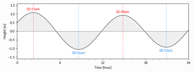
Figure 1.3: Detecting high and low tides
Important
pyTMD uses times in UTC for all calculations [see Time Standards and Time Zones].
Creating a tide table in local time requires applying the appropriate time zone and daylight savings time conversions.