9. Spherical Harmonics

The tide potential at colatitude \(\theta\) and longitude \(\lambda\) is often expressed in terms of spherical harmonic functions \(Y_l^m(\theta,\lambda)\) of degree \(l\) and order \(m\) [17]. These harmonics are solutions of Laplace’s equation in spherical coordinates using separation of variables [29]. The degree 2 spherical harmonic terms are the dominant source of tidal excitation, and induce the semi-diurnal (from \(Y_2^2\)), diurnal (from \(Y_2^1\)) and long-period (from \(Y_2^0\)) tides [61].

Figure 9.1: Spherical harmonics for degree 2

9.1. Mathematical Definition

Spherical harmonics of degree \(l\) and order \(m\) are defined as:

(9.1)\[Y_l^m(\theta, \lambda) = N_l^m\, P_l^m(\cos\theta)\, e^{im\lambda}\]

where \(P_l^m(x)\) are the associated Legendre polynomials and \(N_l^m\) is a normalization factor [29, 50]. pyTMD.math.sph_harm() calculates spherical harmonics using the normalization factor from Equation A5 in Munk et al. [49]. The associated Legendre polynomials of degree \(l\) and order \(m\) are calculated in pyTMD.math.legendre() using the explicit formula (1-67) from Hofmann-Wellenhof and Moritz [29]:

(9.2)\[P_l^m(x) = 2^{-l}(1-x^2)^{m/2}\sum_{k=0}^{n}(-1)^k\frac{(2l-2k)!}{k!(l-k)!(l-m-2k)!}\, x^{l-m-2k}\]

where \(n\) is the largest integer less than or equal to \((l-m)/2\). The first few (unnormalized) Legendre polynomials are:

\(P_0^0(x) = 1\)
\(P_1^0(x) = x\)	\(P_1^1(x) = \sqrt{1-x^2}\)
\(P_2^0(x) = \tfrac{1}{2}(3x^2 - 1)\)	\(P_2^1(x) = 3x\sqrt{1-x^2}\)	\(P_2^2(x) = 3(1-x^2)\)

9.2. Tide-Generating Potential

The gravitational potential \(W\) at a location on Earth’s surface \((\varphi, \lambda)\) from a planetary body (such as the Moon or Sun) can be expanded into spherical harmonics as the following:

(9.3)\[W(\varphi, \lambda) = \frac{G M}{R} \sum_{l=2}^{\infty} \left(\frac{r}{R}\right)^l P_l(\cos\psi)\]

where \(G\) is the gravitational constant, \(M\) is the mass of the body, \(r\) is the radius of the Earth, \(R\) is the distance to the planetary body, and \(\psi\) is the zenith angle between the planetary body and the position on the Earth’s surface [50, 61]. The standard gravitational parameter (\(GM\)) of the planetary body can be derived using that of the Earth (\(GM_E\)) and their ratio of masses (\(M/M_E\)). The cosine of the zenith angle (\(\cos\psi\)) can also be calculated using the dot product between the geocentric unit vectors of the tide-generating body (\(\hat{\mathbf{R}}\)) and the point on the Earth’s surface (\(\hat{\mathbf{r}}\)) [43]:

(9.4)\[\cos\psi = \hat{\mathbf{r}}\cdot\hat{\mathbf{R}} = \frac{\mathbf{r}\cdot\mathbf{R}}{|\mathbf{r}\mathbf{R}|}\]

9.3. Higher-Degree Terms

Global asymmetry in the tide potential can lead to a dependence on higher degree harmonics, most notably the degree 3 and 4 terms. These terms are small compared to those of degree 2, but have been detected at both local and global scales [61]. Both GNSS stations and superconducting gravimeters can be sensitive enough to detect the signals from these higher degree terms [27, 56]. The formalism for computing solid Earth tides within the IERS Conventions include the component of deformation induced by the degree 3 terms [43, 56]. Catalogs of tide potential, such as HW1995 [see Tide Potential Catalogs], can include even higher degree terms, as well as the potentials related to planetary motion [27].

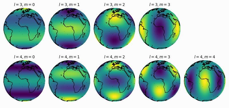
Figure 9.3: Spherical harmonics for degrees 3 and 4

Table 9.1: Maximum Tide Potential from Hartmann and Wenzel [27]

Body	Degree	V [m2/s2]
Moon	2	4.41
Moon	3	7.88×10-2
Moon	4	1.41×10-3
Moon	5	2.53×10-5
Moon	6	4.52×10-7
Moon	7	8.06×10-9
Sun	2	1.60
Sun	3	6.80×10-5
Sun	4	2.89×10-9