Getting Started
Tip
See the Jupyter notebooks and recipes as a quickstart guide for using pyTMD.
Tide Corrections
Different measurement techniques can have different vertical datums, and require different sets of tidal corrections. Tide gauges measure the height of the ocean surface relative to the land upon which they are situated (ocean tides only). Satellite altimeters measure the height of the ocean surface relative to the center of mass of the Earth system (combination of ocean and earth tides).
Application |
Ocean |
Load |
Solid Earth |
Load Pole |
Ocean Pole |
|---|---|---|---|---|---|
Satellite Altimetry |
✔ |
✔ |
✔ |
✔ |
✔ |
Coastal Tide Gauges |
✔ |
✔ |
|||
Grounded GNSS stations |
✔ |
✔ |
✔ |
pyTMD is intended to be able to compute ocean, solid Earth, load and pole tide variations to support the different measurement techniques.
For ocean and load tides, pyTMD uses pre-computed tidal constituent files of amplitude and phase provided by tide modeling groups.
Versions of the following tide models are currently supported [see Choosing a Model]:
Arctic Ocean (AO) and Greenland coast (Gr) tidal simulations [60]
Circum-Antarctic Tidal Simulations (CATS) [61]
Empirical Ocean Tide (EOT) models [31]
Finite Element Solution (FES) tide models [48]
Goddard Ocean Tide (GOT) models [68]
Hamburg direct data Assimilation Methods for Tides (HAMTIDE) models [82]
Technical University of Denmark (DTU) tide models [5]
TOPEX/POSEIDON (TPXO) global tide models [23]
Choosing a Model
pyTMD can access the harmonic constituents for the OTIS, GOT and FES families of ocean and load tide models.
Choosing a model is often a balance between the spatial resolution of the model, the accuracy of the model (e.g. the underlying physics and if it included data assimilation), the number of constituents included in the model, and the geographic region of interest.
Another non-trivial consideration is if the model is openly available for download or if it requires registration and/or manual downloading.
Post on the pyTMD discussions board if you want more information or help choosing a model.
Tide Model Formats
OTIS and ATLAS
OTIS and ATLAS formatted data use binary files to store the constituent data for either heights (z) or zonal and meridional transports (u, v).
They can be either a single file containing all the constituents (compact) or multiple files each containing a single constituent.
ATLAS netCDF formatted data use netCDF4 files for each constituent and variable type (z, u, v).
OTIS and ATLAS binary files can be read via the routines in pyTMD.io.OTIS and ATLAS netCDF files via the routines in pyTMD.io.ATLAS.
GOT
GOT formatted data use ascii or netCDF4 files for each height constituent (z).
Both ascii and netCDF4 files can be read via the routines in pyTMD.io.GOT.
FES
FES formatted data use either ascii (1999, 2004) or netCDF4 (2012, 2014) files for each constituent and variable type (z, u, v).
FES also provides unstructured (“native”) netCDF4 files, which contain data for all constituents on a finite element mesh.
All FES files can be read via the routines in pyTMD.io.FES.
Data Access
Some tide models can be programmatically downloaded using the fetching routines in pyTMD.datasets.
OTIS-formatted Arctic Ocean models can be downloaded from the NSF ArcticData server using the pyTMD.datasets.fetch_arcticdata() function.
GOT models can be downloaded from the NASA GSFC server using the pyTMD.datasets.fetch_gsfc_got() function.
Users registered with AVISO [see Registering with AVISO] can download FES models from their FTP server using the pyTMD.datasets.fetch_aviso_fes() function.
Other tide models may require manual downloading due to licensing agreements or limitations on programmatic access. TPXO models (OTIS and ATLAS formats) can be requested from the data producers after registration. OTIS-formatted Antarctic models are available from the U.S. Antarctic Program Data Center (USAP-DC), which uses a reCAPTCHA security system to prevent automated access. See the model links in Directories for the references to specific tide models.
Model Database
pyTMD comes with a JSON database of models for the prediction of tidal elevations and currents.
An updated version of the database can be downloaded from the project using the pyTMD.datasets.fetch_database() function.
import pyTMD

# create a pyTMD model object from database
m = pyTMD.io.model().from_database("GOT4.10_nc")
m
pyTMD.io.model
name: GOT4.10Directories
pyTMD uses a tree structure for storing and accessing the tidal constituent data.
The base of the tree structure (in the table below as <model_path>) can be the default pyTMD cache directory or a user-specified (external) directory.
The default cache directory is set by the platformdirs package, but can be overridden on a machine by setting the PYTMD_CACHE_DIR environment variable.
The tree structure was chosen based on the different formats of each tide model.
Presently, the following models and their directories are parameterized within pyTMD:
Model |
Directory |
|---|---|
|
|
|
|
|
|
|
|
|
|
|
|
|
|
|
|
|
|
|
|
|
|
|
|
|
|
|
|
|
|
|
|
|
|
|
|
|
|
|
|
|
|
|
|
|
|
|
|
|
|
|
|
|
|
|
|
|
|
|
|
|
|
|
|
|
|
|
|
|
|
|
|
|
|
|
|
|
|
|
|
|
|
|
|
|
|
|
|
|
|
|
|
|
|
|
|
|
|
|
|
|
|
|
|
|
|
|
|
|
|
|
Tip
See Tidal Current Directories for the table of directories for models with tidal currents.
For other tide models, the model parameters can be set with a model definition file.
If you wish to add a new model to the pyTMD database, please see the contribution guidelines.
Note
Any model parameterized with a definition file or added to the database will have to fit a presently supported file standard.
Definition Files
For models not currently within the pyTMD database, the model parameters can be set in pyTMD.io.model with a definition file in JSON format.
The JSON definition files follow a similar structure as the main pyTMD database, but for individual entries.
The JSON format directly maps the parameter names with their values stored in the appropriate data type (strings, lists, numbers, booleans, etc).
While still human readable, the JSON format is both interoperable and more easily machine readable.
Each definition file should have name and format parameters as well as the parameters for the data groups (z, u, v).
Each model type may also require specific sets of parameters for the individual model reader.
For models with multiple constituent files, the files can be found using a glob string to search a directory.
OTIS,ATLAS-compactandTMD3format:OTIS,ATLAS-compactorTMD3name: tide model nameprojection: model spatial projection.z:grid_file: path to model grid filemodel_file: path to model constituent file(s) or aglobstringunits: units of the model constituent data
u:grid_file: path to model grid filemodel_file: path to model constituent file(s) or aglobstringunits: units of the model constituent data
v:grid_file: path to model grid filemodel_file: path to model constituent file(s) or aglobstringunits: units of the model constituent data
ATLAS-netcdfformat:ATLAS-netcdfname: tide model namecompressed: model files aregzipcompressedz:grid_file: path to model grid filemodel_file: path to model constituent files or aglobstringunits: units of the model constituent data
u:grid_file: path to model grid filemodel_file: path to model constituent files or aglobstringunits: units of the model constituent data
v:grid_file: path to model grid filemodel_file: path to model constituent files or aglobstringunits: units of the model constituent data
GOT-asciiandGOT-netcdfformat:GOT-asciiorGOT-netcdfname: tide model namecompressed: model files aregzipcompressedz:model_file: path to model constituent files or aglobstringunits: units of the model constituent data
FES-asciiandFES-netcdfcompressed: model files aregzipcompressedformat:FES-asciiorFES-netcdfname: tide model nameversion: tide model versionz:model_file: path to model constituent files or aglobstringunits: units of the model constituent data
u:model_file: path to model constituent files or aglobstringunits: units of the model constituent data
v:model_file: path to model constituent files or aglobstringunits: units of the model constituent data
FES-nativecompressed: model files aregzipcompressedformat:FES-nativename: tide model nameversion: tide model versionz:model_file: path to model constituent file(s) or aglobstringunits: units of the model constituent data
Units
pyTMD uses pint to handle the units of the model constituent data and convert them into standard sets of units.
z: tidal elevations in meters (\(m\))
u: zonal tidal currents in centimeters per second (\(cm/s\))
U: zonal tidal transports in square meters per second (\(m^2/s\))
v: meridional tidal currents in centimeters per second (\(cm/s\))
V: meridional tidal transports in square meters per second (\(m^2/s\))
pint can also convert the tide prediction data into other sets of units (e.g. feet, knots, etc).
Time
The default time in pyTMD is days (UTC) since a given epoch.
For ocean, load and equilibrium tide programs, the epoch is 1992-01-01T00:00:00.
For pole tide programs, the epoch is 1858-11-17T00:00:00 (Modified Julian Days).
pyTMD uses the timescale library to convert different time formats to the necessary time format of a given program.
timescale can also parse date strings describing the units and epoch of relative times, or the calendar date of measurement for geotiff formats.
Spatial Coordinates
The default coordinate system in pyTMD is WGS84 geodetic coordinates in latitude and longitude.
pyTMD uses pyproj to convert from different coordinate systems and datums.
Some regional tide models are projected in a different coordinate system.
These models have their coordinate reference system (CRS) information stored as PROJ descriptors in the JSON model database:
For other projected models, a formatted coordinate reference system (CRS) descriptor (e.g. PROJ, WKT, or EPSG code) can be used.
Interpolation
For converting from model coordinates, pyTMD uses the linear and nearest spatial interpolation routines from xarray.
Important
If the model domain does not contain the coordinates, the interpolation will return NaN values.
Verify that the coordinates are in the model domain and coordinate reference system.
For coastal or near-grounded points, the model can be extrapolated outside the model domain with pyTMD.interpolate.extrapolate() using a nearest-neighbor (NN) or inverse distance weighting (IDW) algorithm [see Extrapolation Methods].
The default maximum extrapolation distance is 10 kilometers.
This default distance may not be a large enough extrapolation for some applications and models.
Warning
The extrapolation cutoff can be set to any distance (including infinite), but should be used with caution in cases such as estuaries, narrow fjords or ice sheet grounding zones [62].
Programs
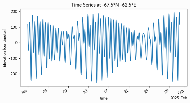
pyTMD.compute calculates tide predictions for use with numpy arrays or pandas dataframes.
These are a series of functions that take x, y, and time coordinates and
compute the corresponding tidal elevation or currents.
import pyTMD
import timescale
import matplotlib.pyplot as plt

lon = -62.5
lat = -67.5
time = timescale.time.date_range("2025-01-01", "2025-01-31", 1, "h")

tide_h = pyTMD.compute.tide_elevations(
    lon,
    lat,
    time,
    model="GOT4.10_nc",
    crs="4326",
    standard="datetime",
    method="linear",
)
model: a tide model available in thepyTMDmodel databasecrs: input coordinate reference system (4326: WGS84 Latitude / Longitude)standard: input time format [see background on time standards]method:xarrayinterpolation method
# update the time coordinate and convert units
tide_h = tide_h.assign_coords(time=time)
tide_h = tide_h.tmd.to_units("cm")
# plot the tide predictions
fig, ax = plt.subplots(
    figsize=(7.5, 3.5),
)
tide_h.plot(ax=ax)
ax.set_ylabel(f"Elevation [{tide_h.units}]")
ax.set_title(f"Time Series at {lat:.1f}°N {lon:.1f}°E")
for label in ax.get_xticklabels(which="major"):
    label.set(rotation=30, horizontalalignment="right")
Data Types
The pyTMD.compute functions accept a type parameter that defines the relationship between the spatial and temporal coordinates and create the output xarray.DataArray dimensions.
The three valid data types in pyTMD are:
'trajectory'When to Use: Spatiotemporal coordinates are arrays of the same length and each element represents a single observation
Typical Applications: drift buoys, ship tracks, airborne or satellite altimetry, instruments that move through space
Output Dimensions:
(time, )
'time series'When to Use: Spatial coordinates are fixed to location(s) and the temporal coordinate is an array of times
Typical Applications: tide gauges, GNSS stations, ocean bottom pressure recorders, moored current meters, instruments that stay in place
Output Dimensions:
(time, )or(station, time)
'grid'When to Use: Spatial coordinates define a 2-dimensional grid and the temporal coordinate is either a scalar or an array of times
Typical Applications: tide maps, raster imagery, satellite imagery, gridded products, model outputs
Output Dimensions:
(y, x)or(y, x, time)
If the type argument is set to None in a pyTMD.compute function, pyTMD.spatial.data_type() will try to auto-detect it based on the dimension sizes.
Tip
See the background material and glossary for more information on the theory and methods.