10. Love and Shida Numbers
When the Moon or Sun exerts a tidal force on the Earth, the solid body of the Earth deforms both elastically and inelastically [see Solid Earth Tides]. This deformation has three distinct components:
a vertical (radial) displacement of the surface
a horizontal (tangential) displacement of the surface
a change in the gravitational potential
The magnitude of each individual component can be characterised by a dimensionless scaling factor [46, 77]. These factors are collectively known as Love/Shida Numbers, and are defined for each spherical harmonic degree.
Symbol |
Name |
|---|---|
\(h_l\) |
Love number (vertical) |
\(k_l\) |
Love number (potential) |
\(l_l\) |
Shida number (horizontal) |
10.1. Tidal Love Numbers
Tidal-effective Love numbers describe the deformation of the solid Earth in response to the direct gravitational potential of a remote body (such as the Sun or Moon). The tidal forcing is distributed throughout the entirety of the Earth’s volume [59].
Elastic Love numbers assume that the Earth responds instantaneously to the tidal forcing and without any dissipation. For a spherical, non-rotating Earth, the Love/Shida numbers are largely independent of tidal frequency as the tidal periods are longer than the Earth’s free oscillation periods [6, 88, 89]. However, for a rotating, ellipsoidal Earth, the Love/Shida numbers have some dependence on tidal frequency, with resonances particularly in the diurnal band [42, 69, 88, 89].

Figure 10.1: Diurnal frequency dependence of Love/Shida numbers from Wahr [88]
Additionally, the Earth’s mantle is not perfectly elastic, and there is a small phase lag between the tidal forcing and the deformation response.
Complex Love numbers contain a real part describing the in-phase (elastic) response and an imaginary part describing the out-of-phase (dissipative) response [65, 89].
pyTMD computes both the frequency-dependent corrections and the dissipative responses following Mathews et al. [51] and Wahr [89].
Combinations of Love/Shida numbers can derive additional quantities [6, 13, 24, 55, 59]:
Name |
Expression |
|---|---|
\(\delta_l = 1 + \dfrac{2h_l}{l} - \dfrac{(l + 1)k_l}{l}\) |
|
\(\gamma_l = 1 + k_l - h_l\) |
pyTMD uses these factors in a few different computations, including the calculation of long-period equilibrium tides, ocean pole Tides and gravity tides.
Similar to the original Love/Shida numbers, the tidal factors will have a dependence on tidal frequency [88] and contain imaginary components for the dissipative response [89].
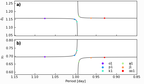
Figure 10.3: Diurnal frequency dependence of the gravimetric and tilt factors
10.2. Load Love Numbers
Load Love numbers describe the deformation of the solid Earth in response to a change in surface mass load. The loading change, such as from a redistribution ocean mass from tides, acts upon the surface of the Earth [87]. These “load tides” are computed through a convolution of the tidal constituents and load Love numbers typically by either a Green’s function or spherical harmonic approach [2, 25]. In either of those cases, the calculation uses a set of load Love numbers to high spherical harmonic degree.