Extrapolation Methods

This notebook demonstrates using the extrapolation methods contained in pyTMD:

• NN: Nearest-Neighbors

• IDW: Inverse-Distance Weighting

• DCT: Discrete-Cosine Transform Inpainting

import numpy as np
import xarray as xr
import pyTMD.interpolate
import matplotlib.pyplot as plt

Franke’s bivariate test function

def franke(x, y):
    F1 = 0.75 * np.exp(-((9.0 * x - 2.0) ** 2 + (9.0 * y - 2.0) ** 2) / 4.0)
    F2 = 0.75 * np.exp(-((9.0 * x + 1.0) ** 2 / 49.0 - (9.0 * y + 1.0) / 10.0))
    F3 = 0.5 * np.exp(-((9.0 * x - 7.0) ** 2 + (9.0 * y - 3.0) ** 2) / 4.0)
    F4 = 0.2 * np.exp(-((9.0 * x - 4.0) ** 2 + (9.0 * y - 7.0) ** 2))
    F = F1 + F2 + F3 - F4
    return F

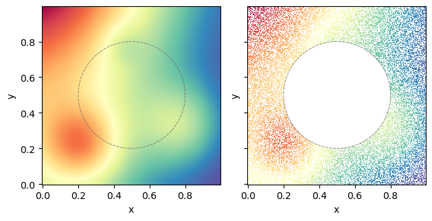
Create a smooth grid with missing values

# calculate output points
ny, nx = 250, 250
# normalized grid points
xpts = np.arange(nx) / np.float64(nx)
ypts = np.arange(ny) / np.float64(ny)
XI, YI = np.meshgrid(xpts, ypts)
# calculate real values at grid points
ZI = xr.DataArray(franke(XI, YI), coords=dict(y=ypts, x=xpts), dims=["y", "x"])

# create random points to be removed from the grid
rng = np.random.default_rng(0)
indx = rng.integers(0, high=nx, size=50000)
indy = rng.integers(0, high=ny, size=50000)
# create copy of grid with random points removed
da = ZI.copy()
da.values[indy, indx] = np.nan
# remove a circle of points in the middle of the grid
xc, yc, R = (0.5, 0.5, 0.3)
da = da.where((da.x - xc) ** 2 + (da.y - yc) ** 2 > R**2)
# x and y points along the circle of missing data
xi, yi = pyTMD.ellipse._xy(major=R, minor=R, incl=0.0, xy=(xc, yc), N=100)

# create plot with original and missing data
f1, ax1 = plt.subplots(num=1, ncols=2, sharex=True, sharey=True)
ZI.plot(ax=ax1[0], cmap="Spectral_r", add_colorbar=False)
da.plot(
    ax=ax1[1],
    vmin=ZI.min(),
    vmax=ZI.max(),
    cmap="Spectral_r",
    add_colorbar=False,
)
for ax in ax1:
    ax.plot(xi, yi, color="0.4", ls="--", lw=0.5, dashes=[6, 2])
    ax.set_aspect("equal", "box")
f1.tight_layout();

Extrapolate data to missing values

indices = np.isnan(da.values)
# create copies of the data array for each interpolation method
NN = da.copy()
IDW = da.copy()
DCT = da.copy()
# extrapolate missing values
NN.values[indices] = pyTMD.interpolate.extrapolate(
    da.x,
    da.y,
    da.values,
    XI[indices],
    YI[indices],
    k=1,
    is_geographic=False,
    workers=-1,
)
IDW.values[indices] = pyTMD.interpolate.extrapolate(
    da.x,
    da.y,
    da.values,
    XI[indices],
    YI[indices],
    k=1000,
    is_geographic=False,
    workers=-1,
)
DCT.values[:] = pyTMD.interpolate.inpaint(
    da.x,
    da.y,
    da.values,
    N=100,
    is_geographic=False,
    workers=-1,
)
# calculate absolute difference between extrapolated and original data
dNN = np.abs(NN - ZI)
dIDW = np.abs(IDW - ZI)
dDCT = np.abs(DCT - ZI)

# create plot with extrapolation results and differences
f2, ax2 = plt.subplots(num=2, nrows=2, ncols=3, sharex=True, sharey=True)
# plot extrapolated data
titles = ["NN", "IDW", "DCT"]
kwargs = dict(
    vmin=ZI.min(),
    vmax=ZI.max(),
    cmap="Spectral_r",
    add_colorbar=False,
    add_labels=False,
    xticks=[],
    yticks=[],
)
NN.plot(ax=ax2[0, 0], **kwargs)
IDW.plot(ax=ax2[0, 1], **kwargs)
DCT.plot(ax=ax2[0, 2], **kwargs)
for ax, title in zip(ax2[0], titles):
    ax.plot(xi, yi, color="0.4", ls="--", lw=0.5, dashes=[6, 2])
    ax.set_aspect("equal", "box")
    ax.set_title(title)
# plot absolute difference between extrapolated and original data
titles = ["NN diff", "IDW diff", "DCT diff"]
kwargs.update(vmin=dNN.min(), vmax=dNN.max(), cmap="PuBuGn")
dNN.plot(ax=ax2[1, 0], **kwargs)
dIDW.plot(ax=ax2[1, 1], **kwargs)
dDCT.plot(ax=ax2[1, 2], **kwargs)
for ax, title in zip(ax2[1], titles):
    ax.plot(xi, yi, color="0.4", ls="--", lw=0.5, dashes=[6, 2])
    ax.set_aspect("equal", "box")
    ax.set_title(title)
# adjust layout
f2.tight_layout();

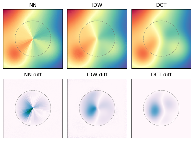
Important

DCT inpainting works well in this example because our evaluation function is smooth. In reality, shallow-water tide effects and other modulations will greatly impact calculations in coastal areas. Extrapolating tides beyond a model’s boundaries should always be done with caution!