Plot Ocean Pole Tide Map

This notebook demonstrates plotting maps of the real and imaginary geocentric pole tide admittance functions from Desai et al. (2002)

• IERS map of ocean pole tide coefficients

Python Dependencies

• cartopy: Python package designed for geospatial data processing

• matplotlib: Python 2D plotting library

• numpy: Scientific Computing Tools For Python

• xarray: N-D labeled arrays and datasets in Python

Program Dependencies

• io.IERS: Read ocean pole load tide map from IERS

• utilities.py: download and management utilities for files

Load modules

import matplotlib.pyplot as plt
import matplotlib.colors as mcolors
import cartopy.crs as ccrs
import pyTMD.io

Read ocean pole tide coefficient maps

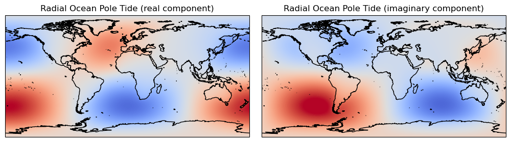
# read ocean pole tide map from Desai (2002)
ds = pyTMD.io.IERS.open_dataset()

Plot ocean pole tide maps

fig, ax = plt.subplots(
    ncols=2,
    sharex=True,
    sharey=True,
    figsize=(10, 4),
    subplot_kw=dict(projection=ccrs.PlateCarree()),
)
# use a centered normalization around zero
norm = mcolors.CenteredNorm(vcenter=0.0)
# plot real and imaginary components
ds["R"].real.plot(
    ax=ax[0], add_labels=False, add_colorbar=False, norm=norm, cmap="coolwarm"
)
ds["R"].imag.plot(
    ax=ax[1], add_labels=False, add_colorbar=False, norm=norm, cmap="coolwarm"
)
# adjust plot details
for i, comp in enumerate(["real", "imaginary"]):
    ax[i].set_title(f"Radial Ocean Pole Tide ({comp} component)")
    # add moderate resolution cartopy coastlines
    ax[i].coastlines("50m")
    # set global view
    ax[i].set_global()
# adjust layout and show
fig.subplots_adjust(left=0.01, right=0.99, bottom=0.10, top=0.95, wspace=0.05)
plt.show()